← go back
VROOOOOOOM
Fast RISC-V GEMMs and Kernel Fusion
july 4 2024
This summer, I devoured this fantastic RISC-V computer architecture textbook and it totally expanded my understanding of how computers work. Prior to reading, I came from a heavy SWE background, and this textbook did a great job of explaining the hardware-software interface. It was the first time I learned about low-level hardware, processor design, and RISC (shoutout 1995 Hackers) , so it got me to start appreciating how much goes into making computers end-to-end.
At the end of each chapter of the textbook, they incrementally show how to make a matrix multiply fast, eventually speeding up by 44,226x over a purely Python implementation. I thought it would be interesting to look into incrementally improving General Matrix Multiplies (GEMMs) with RISC-V CPUs and all sorts of interesting ways to optimize neural network inference with computation graph techniques with GPUs/TPUs.
Table of Contents:
1. Tiny Transistors
2. GPUs and AI Accelerators
3. Graph Rewrite and Kernel Fusion
4. GEMM: Pure Python
5. GEMM: Pure C + Column-Major Array
6. GEMM: Data-Level Parallelism, Sub-Word Parallelism, x86 AVX, and ARM Neon
7. GEMM: Instruction level Parallelism
8. GEMM: Memory Hierarchy Optimization
9. GEMM: Thread level Parallelism
10. JIT Compilation
11. References
1. Tiny Transistors
Computers are fast. Both software and hardware have benefited from Moore's Law since 1965. Moore's law is slowing, but that doesn't mean that computers won't improve much. In fact, we can still expect a 1,000,000x shrinkage of transistor size alone. Jim Keller explains it well in that a modern transistor is about 1000x1000x1000 atoms wide. We start experiencing weird quantum effects at around 10 atoms, so we can still get a times smaller transistor. Smaller transistor sizes create smaller gate capacitance and lower operating voltages, which allow faster switching times. It's mind-boggling, but clock speeds could be thousands to millions of times faster, only limited by the speed of light for signal propagation. The future will be amazing.
2. GPUs and AI Accelerators
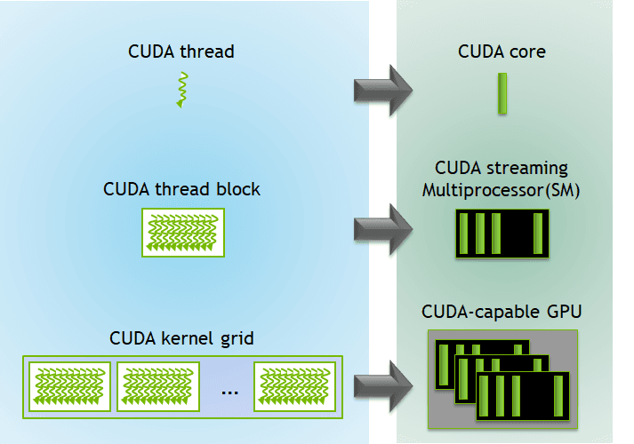
First, a brief overview of GPU architecture. Kernels are functions on GPUs that are ran in parallel on multiple threads. Threads are individual units of execution on a GPU. There are 32 threads in a warp, which is the smallest unit of execution that you can call. You can combine many warps into a block, which makes up a grid.

GPUs have many streaming multiprocessors (AMD has a better name for these, Compute Units) that contain a scheduler, shared memory, and SIMD vector processors. Branch Education has a video with amazing visualizations explaining how GPUs work. I highly recommend watching it.
NVIDIA's flagship consumer GPU is the RTX 4090. It has 16,384 CUDA cores, which can execute an FMA in one clock cycle. With 16,384 cores, 2 calculations per core, 2.5 GHz clock, we get about 82.58 FP32 TFLOPS. Compare this to an i9-13900K, which does 2.5 FP32 TFLOPS, 33x slower than the 4090. This is because, in general, GPUs trade off massive throughput for high latency.
NVIDIA offers a programming model that uses GPUs for general-purpose computing, where you can write custom kernels. Simon Boehm has a world-class resource for optimizing GEMMs on NVIDIA GPUs using CUDA.
Another way to speed up GEMMs is by creating hardware specialized for common operations in neural networks called AI accelerators. Some examples are Google TPU, Tenstorrent Grayskull, Apple Neural Engine, Tesla Dojo, and Meta MTIA.

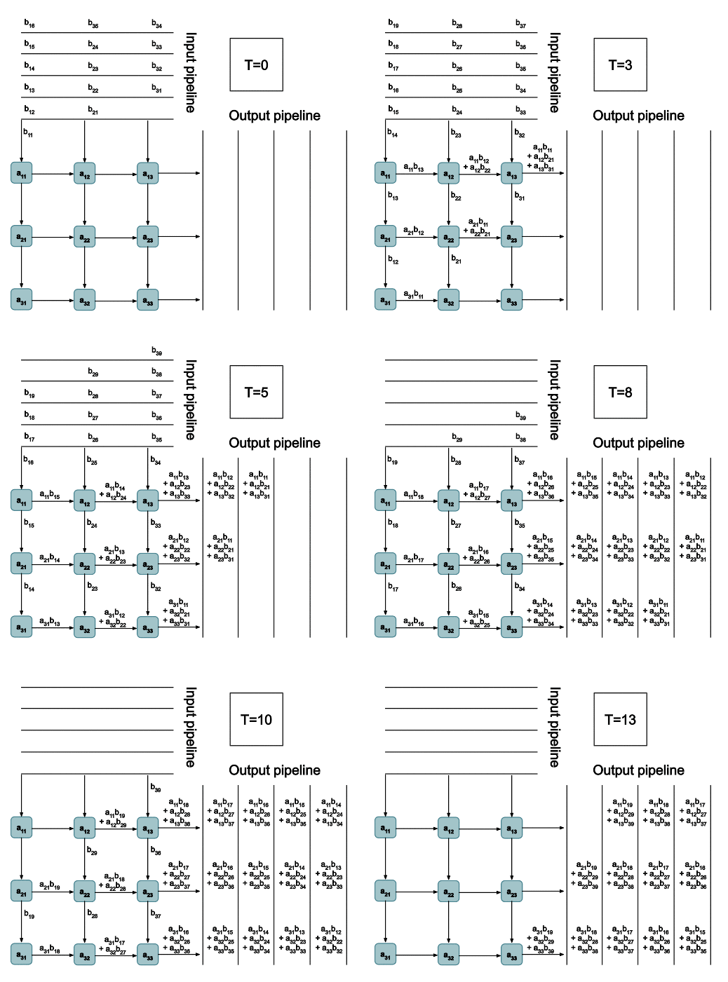
The TPUv2 chip is once of the AI accelerator ASICs that we talked about earlier. The architecture is super interesting and it uses systolic arrays (shown below) to do matrix multiplications:
3. Graph Rewrite and Kernel Fusion
If you look at Meta's blog post about MTIA v1, you'll notice they mention two different modes of execution for PyTorch: eager mode and graph mode.
Operators in eager mode execute ASAP once encountered. This is great for fast development and is the default mode of execution. There's also graph mode which translates operations into a graph that can then be optimized for high performance, similar to the JIT compiler that we talked about earlier.
With graph mode, we model computation as a graph where mathematical operations are nodes and dependencies are the edges. Using this abstraction, you can imagine a neural network, with all its mathematical operations, modeled as a graph of computation, like the one below.
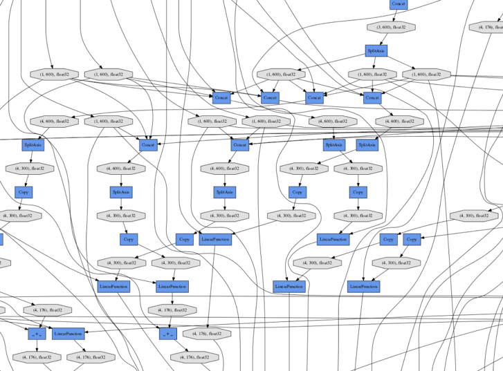
Through analysis of this graph, there are special techniques like kernel fusion, which optimizes the performance of networks by merging nodes together. This helps performance by reducing memory reads and kernel overhead. This optimization of graphs is a general technique called graph rewriting.
First, there is "operation fusion," where two operations are merged together. Operator fusion has two dimensions: horizontal and vertical. Horizontal fusion takes a single operation that is independently applied to many operands (SIMD...) and merges the operations into a single array.
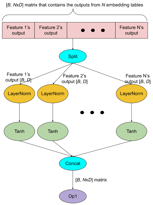
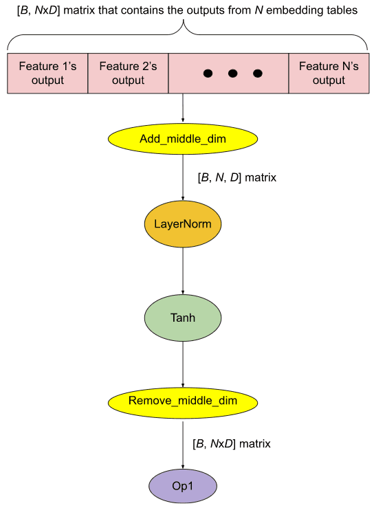
As an example of horizontal fusion, here are two graphs from the PyTorch blog that illustrate horizontal fusion in a real network.
On the other hand, vertical fusing merges a kernel that takes another kernels output both into one. For example, take two kernels A and B:
vertically fusing C and D results in:
GPUs are heavily constrained by latency to memory which it hides through an insane amount of threads. Each thread then runs a kernel which has overhead to load into memory and run. Operator fusion minimizes this overhead by combining multiple data operations into one. One caveat: this doesn't work in eager mode, which is PyTorch's default execution mode. This is why they introduced torch.compile, which allows for JIT compilation and all this overhead to be minimized by the compiler.
You can learn more about real-world kernel fusion through PyTorch, CUDA Graphs, NVIDIA cuDNN, and tinygrad.
Since neural net operations are defined beforehand as graphs, they are essentially just predetermined static loops of computation. Future frameworks and ML compilers will have really awesome opportunities to take advantage of this and innovate in areas like:
- Dynamic scheduling: optimizing resource allocation and execution order in real-time
- Adaptive graph rewrites: automatically restructuring computational graphs for improved performance
- Compilation techniques: developing more sophisticated methods for easier translation of high-level models into highly optimized low-level code for all accelerators
4. GEMM: Pure Python
Matrix multiplication is the fundamental operation of computation for modern-day deep learning. Trillions and trillions of matrix multiplies can happen each second during each pass of a neural network, so speeding up GEMMs, even just a little but can save lots of money and time, resulting in a massive impact in iteration speeds for developers.
Remember matrix-matrix multiplication from linear algebra? Thats a GEMM -- an accumulation of matrix-matrix multiplies. More formally,
What does it look like in code?
for i in range(M):
    for j in range(N):
        for k in range(K):
            C[i][j] += A[i][k] * B[k][j]
The above code, in Python, is pretty much the simplest GEMM you can write. We take two matrices, A and B, and create a matrix C. We then loop over each i, j, with an extra k loops to do a succession of dot products.
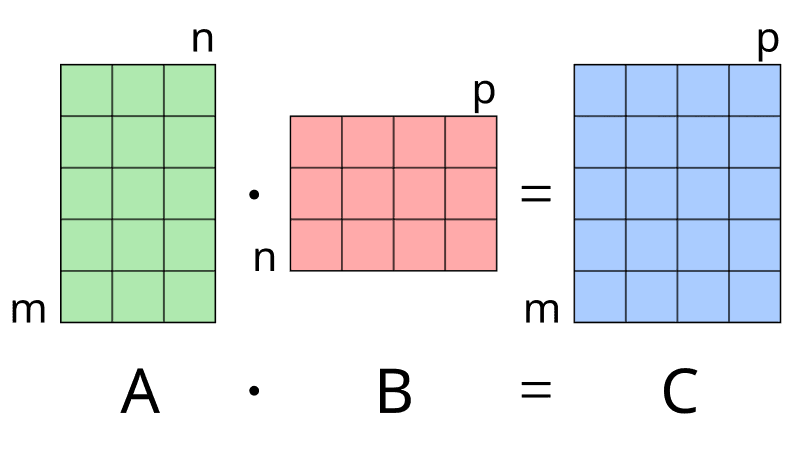
The photo above shows the dimensions of a GEMM where p == k. The really important thing to notice is that C[i][j] += A[i][k] * B[k][j]. This is the common formula for all GEMMs.
Running this GEMM produces a mean execution time of 0.127866 seconds and a standard deviation of 0.030468 seconds. This will be our baseline against which to compare future speedups.
5. GEMM: Pure C + Column-Major Array
void dgemm(int n, double* A, double* B, double* C)
{
    for (int i = 0; i < n; ++i) {
        for (int j = 0; j < n; ++j) {
            double cij = C[i+j*n];          /* cij = C[i][j] */
            for (int k = 0; k < n; k++)
                cij += A[i+k*n] * B[k+j*n]; /* cij += A[i][k]*B[k][j] */
            C[i+j*n] = cij;                 /* C[i][j] = cij */
        }
    }
}
We take in int n since we are multiplying NxN matrices. We also pass pointers to our A, B, and C matrices. Overall, we have only changed two concepts in the code above. First, we have switched the code to C. Under the hood, Python is implemented with CPython so we can increase speed by skipping over the Python interpreter and getting general benefits from a compiled language, as mentioned in section 8. We can also get a speedup by converting our output matrix into a 1D array using column-major order.
Column Major Order:

We can further understand the operations by realizing that:
A[i+k*n] represents A[i][k]B[k+j*n] represents B[k][j]C[i+j*n] represents C[i][j]By squashing the matrix into column-major order and doing a straightforward mapping to find the index, consecutive accesses to elements of a single column in B result in more efficient memory access patterns due to spatial locality and increased cache performance.
You might have also noticed that we called the function dgemm. In case you were wondering, this means double precision matrix multiplies.
How does this compare to pure Python? Using no compiler optimization, this gets a 77x speedup!
6. GEMM: Data-Level Parallelism, Sub-Word Parallelism, x86 AVX, and ARM Neon
Data-level parallelism is the method of increasing throughput by using a single instruction operation on multiple data (SIMD) simultaneously. Differently, sub-word parallelism is a specific form of data-level parallelism where you divide a word into subwords and operate on them parallelly. The dgemm function provided uses both data-level parallelism and subword parallelism. We will write a DGEMM that employs Advanced Vector Extensions (AVX) instructions to perform the same operations on subwords in parallel, utilizing the capabilities of SIMD architecture to speed up GEMMs.
//include <x86intrin.h>
void dgemm(size_t n, double* A, double* B, double* C)
{
    for (size_t i = 0; i < n; i += 4) {
        for (size_t j = 0; j < n; j++) {
            __m256d c0 = _mm256_load_pd(C+i+j*n);           /* c0 = C[i][j] */
            for (size_t k = 0; k < n; k++) {
                c0 = _mm256_add_pd(c0,                      /* c0 += A[i][k]*B[k][j] */
                    _mm256_mul_pd(_mm256_load_pd(A+i+k*n),
                        _mm256_broadcast_sd(B+k+j*n))
                );
            }
            _mm256_store_pd(C+i+j*n, c0);                   /* C[i][j] = c0 */
        }
    }
}
The code above utilizes Advanced Vector Extensions (AVX), which are SIMD extensions to the x86 instruction set architecture (ISA). We include the header #include <x86intrin.h> and use the __m256d type. This type represents a 256-bit wide vector that holds four double-precision floating-point numbers (each 64 bits).

As a result, we process four doubles simultaneously in each iteration. The outer loop iterates in steps of four because each step loads four double-precision values (64 bits each, totaling 256 bits).
We assign this to _mm256_load_pd(C+i+j*n), "Moves packed double-precision floating point values from aligned memory location to a destination vector". The command _mm256_broadcast_sd is very interesting in that we first see the concept of broadcasting. Broadcasting takes the smaller array and repeats it so that two matrices have the same shape and can be matmul'd.
Let's look at broadcasting a bit more closely with NumPy:
a = np.array([1.0, 2.0, 3.0])
b = 2.0
a * b
>>> array([2.,  4.,  6.])
a is shape of (3,1) while b is a double with size (1,).
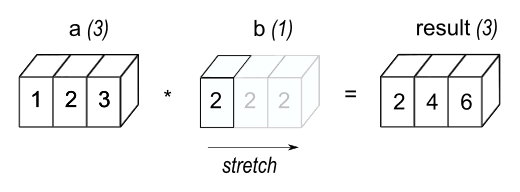
We can "unify" these shapes by extending b into a shape of (3,1) with repeated 2.0's, as seen above. In the operation above, b was "broadcasted".
Back in the code, we see different address translation calculations. Don't worry, everything is still column-major stored where C+i+j*n just represents C[i+j*n] . Using AVX speeds up our GEMM by an additional 7.8x, which we might expect by issuing multiple operations at a time.
The AVX code above uses special vector extensions to x86. unfortunately, I'm on an ARM Macbook. We can rewrite the code using Advanced SIMD (aka ARM Neon) intrinsics:
#include <arm_neon.h>

void dgemm(size_t n, double* A, double* B, double* C) {
    for (size_t i = 0; i < n; i += 2) {
        for (size_t j = 0; j < n; j++) {
            float64x2_t c0 = vld1q_f64(C + i + j*n);      // Load the current values of C into vector c0
            for (size_t k = 0; k < n; k++) {
                float64x2_t a = vld1q_f64(A + i + k*n);   // Load two values from matrix A into vector a
                float64x2_t b = vdupq_n_f64(B[k + j*n]);  // Duplicate the value B[k + j*n] into all elements of vector b
                c0 = vfmaq_f64(c0, a, b);                 // Perform the fused multiply-add operation
            }
            vst1q_f64(C + i + j*n, c0);                   // Store the result back into matrix C
        }
    }
}
You should be able to get the gist of the code by now. We can see that we #include <arm_neon.h>. float64x2_t is an ARM specific 128-bit wide vector (consists of two 64-bit floats). vld1q_f64 loads multiple single-element structures to one, two, three, or four registers. You can now have a GEMM that uses data-level parallelism on your ARM device!
7. GEMM: Instruction level Parallelism
#include <x86intrin.h>
#define UNROLL (4)

void dgemm(int n, double* A, double* B, double* C)
{
    for (int i = 0; i < n; i += UNROLL * 8)
        for (int j = 0; j < n; ++j) {
            __m512d c[UNROLL];
            for (int r = 0; r < UNROLL; r++)
                c[r] = _mm512_load_pd(C + i + r * 8 + j * n);
            for (int k = 0; k < n; k++) {
                __m512d bb = _mm512_broadcastsd_pd(_mm_load_sd(B + j * n + k));
                for (int r = 0; r < UNROLL; r++)
                    c[r] = _mm512_fmadd_pd(_mm512_load_pd(A + n * k + r * 8 + i), bb, c[r]);
            }
            for (int r = 0; r < UNROLL; r++)
                _mm512_store_pd(C + i + r * 8 + j * n, c[r]);
        }
}#include <arm_neon.h>
void dgemm(int n, double* A, double* B, double* C)
{
for (int i = 0; i < n; i += UNROLL * 2)
for (int j = 0; j < n; ++j) {
float64x2_t c[UNROLL];
for (int r = 0; r < UNROLL; r++)
c[r] = vld1q_f64(C + i + r * 2 + j * n);
for (int k = 0; k < n; k++) {
float64x2_t bb = vdupq_n_f64(B[j * n + k]);
for (int r = 0; r < UNROLL; r++)
c[r] = vfmaq_f64(c[r], vld1q_f64(A + n * k + r * 2 + i), bb);
}
for (int r = 0; r < UNROLL; r++)
vst1q_f64(C + i + r * 2 + j * n, c[r]);
}
}Here are two distinct GEMM implementations, one optimized for AVX and the other for ARM architectures. The macro #define UNROLL specifies the loop unrolling factor, which increases the granularity of the loop iterations and facilitates instruction-level parallelism. Loop unrolling enables the processor to issue more instructions per cycle, particularly advantageous for out-of-order execution processors. These processors can execute instructions in a different sequence from their appearance in the program's source code, enhancing performance. By utilizing multiple execution units and keeping CPU pipelines fully utilized, loop unrolling significantly boosts overall performance.
Compared to the pure Python version, these DGEMMs are 4600x times faster.
8. GEMM: Memory Hierarchy Optimization
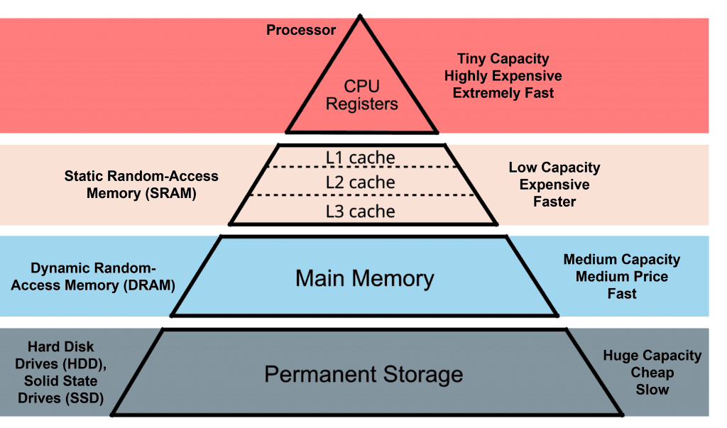
One of the critical concepts in optimizing performance is memory hierarchy. It differs, but each computer has a memory hierarchy with differing speed and capacity levels. As you go down the hierarchy, both size and latency increase.
| Memory Type | Latency | Typical Capacity |
|---|---|---|
| Register | ~1 cycle | In RISC-V: 32 registers, each 32 bits wide |
| L1 Cache | ~1-3 cycles (1ns) | 32KB - 128KB |
| L2 Cache | ~10-20 cycles (4ns) | 256KB - 1MB |
| L3 Cache | ~30-50 cycles | 2MB - 32MB |
| RAM | ~100-200 cycles (100ns) | 8GB - 32GB |
| SSD | ~10,000-100,000 cycles (16,000ns) | 32GB - 8TB |
| HDD | ~1,000,000 cycles (470,000ns) | 64GB - 20TB |
| Cloud Storage | ~10,000,000 cycles | Virtually unlimited |
Having to load and store from main memory (or even worse from storage) forces the computer to stall operations for an insanely long time, so memory management must be done right.
Cache blocking (aka loop blocking or loop tiling) is a technique for improving cache usage. The primary idea is to divide a large chunk of compute into smaller sub-problems (blocks) that fit into the cache. By working on smaller blocks, the program can keep the data in the faster cache memory for longer periods, reducing the number of slow main memory accesses. Let's add this to our GEMM.
#include <x86intrin.h>
#define UNROLL (4)
#define BLOCKSIZE 32

void do_block(int n, int si, int sj, int sk, double *A, double *B, double *C)
{
    for (int i = si; i < si + BLOCKSIZE; i += UNROLL * 8)
        for (int j = sj; j < sj + BLOCKSIZE; j++) {
            __m512d c[UNROLL];
            for (int r = 0; r < UNROLL; r++)
                c[r] = _mm512_load_pd(C + i + r * 8 + j * n);
            for (int k = sk; k < sk + BLOCKSIZE; k++) {
                __m512d bb = _mm512_broadcastsd_pd(_mm_load_sd(B + j * n + k));
                for (int r = 0; r < UNROLL; r++)
                    c[r] = _mm512_fmadd_pd(_mm512_load_pd(A + n * k + r * 8 + i), bb, c[r]);
            }
            for (int r = 0; r < UNROLL; r++)
                _mm512_store_pd(C + i + r * 8 + j * n, c[r]);
        }
}

void dgemm(int n, double* A, double* B, double* C)
{
    for (int sj = 0; sj < n; sj += BLOCKSIZE)
        for (int si = 0; si < n; si += BLOCKSIZE)
            for (int sk = 0; sk < n; sk += BLOCKSIZE)
                do_block(n, si, sj, sk, A, B, C);
}
To improve cache utilization, we define BLOCKSIZE as 32, which creates a 32x32 block. We then loop unroll 4 iterations, and then use AVX-512 intrinsics to perform operations on multiple data points simultaneously, as seen before. The _mm512_fmadd_pd operation does a fused multiply-add, which is an addition and multiplication in a single instruction.
The do_block function does multiplication for a single block, processing 8 double precision floats at once (8x64=512).
#include <riscv_vector.h>

void do_block(int n, int si, int sj, int sk, double *A, double *B, double *C)
{
    for (int i = si; i < si + BLOCKSIZE; i += 8) {
        for (int j = sj; j < sj + BLOCKSIZE; j++) {
            vfloat64m8_t c = vle64_v_f64m8(C + i + j * n, 8);

            for (int k = sk; k < sk + BLOCKSIZE; k++) {
                vfloat64m8_t a = vle64_v_f64m8(A + n * k + i, 8);
                vfloat64m1_t b = vfmv_v_f_f64m1(B[j * n + k], 8);
                c = vfmadd_vv_f64m8(a, b, c, 8);
            }

            vse64_v_f64m8(C + i + j * n, c, 8);
        }
    }
}
We can simply modify do_block to use RISC intrinsics. You can learn more about these functions through GCC.
In conclusion, performance increases are a function of how much memory you have. Since small matrices fit inside the l1 cache, cache blocking makes little difference. However, we can see significant increases up to 10x for huge matrices.
9. GEMM: Thread level Parallelism
#include <x86intrin.h>
#define UNROLL (4)
#define BLOCKSIZE 32

void do_block(int n, int si, int sj, int sk, double *A, double *B, double *C)
{
    for (int i = si; i < si + BLOCKSIZE; i += UNROLL * 8)
        for (int j = sj; j < sj + BLOCKSIZE; j++) {
            __m512d c[UNROLL];
            for (int r = 0; r < UNROLL; r++)
                c[r] = _mm512_load_pd(C + i + r * 8 + j * n);
            for (int k = sk; k < sk + BLOCKSIZE; k++) {
                __m512d bb = _mm512_broadcastsd_pd(_mm_load_sd(B + j * n + k));
                for (int r = 0; r < UNROLL; r++)
                    c[r] = _mm512_fmadd_pd(_mm512_load_pd(A + n * k + r * 8 + i), bb, c[r]);
            }
            for (int r = 0; r < UNROLL; r++)
                _mm512_store_pd(C + i + r * 8 + j * n, c[r]);
        }
}

void dgemm(int n, double* A, double* B, double* C)
{
    #pragma omp parallel for
    for (int sj = 0; sj < n; sj += BLOCKSIZE)
        for (int si = 0; si < n; si += BLOCKSIZE)
            for (int sk = 0; sk < n; sk += BLOCKSIZE)
                do_block(n, si, sj, sk, A, B, C);
}
The old but trusty OpenMP makes an appearance! We can simply use #pragma omp parallel to get a great speedup which allows us to parallelize for loops. It distributes the loop iterations over different threads, which allows us to actually use our multi-core processors. OpenMP is really easy to use, and depending on the number of cores, you can expect performance increases by a factor of 3-4 OOMs.

Here's a great image from the RISC-V computer architecture textbook that shows GEMM performance improvement relative to the number of threads. CPU manufacturers have been pushing single-core processors to the limits, and we started getting diminishing returns, so the easiest way to keep increasing performance was to combine many processors together. Developers then had to start learning about making code parallelizable to ensure that code takes advantage of multiple cores.
To recap, we have worked our way up to a very fast GEMM, improving runtime performance by orders of 4-5 OOMs with:
- Python, C, data-level parallelism, sub-word parallelism, x86 AVX, ARM Neon, instruction-level parallelism, memory hierarchy optimization with cache blocking, and thread-level parallelism.
Eventually, we will encounter decreasing returns through multi-processing and will have to start considering domain-specific architectures (ahem...GPUs) and languages to keep realizing impressive performance increases.
10. NumPy + JIT Compilation
In reality, the easiest way to get out-of-the-box performance is to simply just use NumPy.
import numpy as np

def matrix_multiply(A, B):
    A = np.array(A)
    B = np.array(B)
    return np.dot(A, B)
NumPy is blazingly fast. We get a mean execution time of 0.001728 seconds and a standard deviation of 0.002820 seconds.
This is a 73.9965277778 time improvement! Pretty easy right? Maybe a bit too easy...let's understand why NumPy is so fast.
Dynamic languages (Python, Javascript, and Ruby) infamously have loops and function calls that are extremely slow. These languages determine the types of variables at runtime, which adds a lot of overhead compared to statically typed languages. In addition, these languages are often interpreted line-by-line. This is a lot slower than a compiled language which just executes precompiled machine code.
One way to increase performance is through something called a Just In Time (JIT) compiler.
A JIT compiler is a program that turns bytecode (a portable intermediate representation of the source code) directly into instructions that can be sent directly to the CPU while the program is running. JIT compilers identify "hot spots" in the code, which are sections that are executed frequently, such as loops and heavily used functions. By focusing on these hot spots, JIT compilers can apply aggressive optimizations to improve performance significantly. For example, the JIT can generate machine code for loop variables whose type always stays as an integer. JITs actually need to be warmed up because they need to analyze the code and optimize it. This means that the initial execution of loops and function calls will be slow until the JIT has had time to optimize the code path.
In the background, NumPy utilizes several techniques for fast performance. First, it discards Python lists entirely and defines a custom data structure, numpy.array. numpy.array is fast because it is a densely packed list of homogenous elements stored in contiguous chunks of memory. This contrasts with elements in vanilla Python lists, which are a list of pointers to objects. This is what allows non-homogenous elements to be in a single Python list.
This special numpy.array can take advantage of many other techniques, especially parallelism and multi-threading. If you need a refresher, multi-threaded operations use multiple CPU cores to execute instructions in parallel. NumPy can use Single Instruction Multiple Data (SIMD) to enforce homogenous arrays. SIMD allows a single CPU instruction to operate on multiple data simultaneously. As we will see later, you can also do parallel execution very efficiently through vector processors, whose typical example is the GPU since it specializes in vector calculations.
As we saw above, NumPy uses broadcasting, which allows operations to be performed on arrays of different shapes without making explicit copies of data. Third, NumPy functions aren't actually implemented in Python; instead, they are implemented in C and Fortran. This offloading to C and Fortran minimizes Python's interpreter overhead. NumPy functions are also already pre-compiled into machine code so that they can run instantly.
Overall, none of this stuff is super fancy. It's just using classic computer science optimization techniques. Parallelism, multithreading, adding large buffers, and efficient memory allocation are all general techniques used to improve program performance.
11. References
- NVIDIA: Matrix Multiplication Background User's Guide
- NVIDIA: cuDNN Graph API
- Simon Boehm: How to Optimize a CUDA Matmul Kernel for cuBLAS-like Performance
- PyTorch: Optimizing Production PyTorch Models' Performance with Graph Transformations
- Arxiv: DNNFusion Accelerating Deep Neural Networks Execution with Advanced Operator Fusion
- Stephen Wolfram: Finally We May Have a Path to the Fundamental Theory of Physics… and It's Beautiful
- Tinygrad Notes: How Kernel Fusion Starts
- Horace He: Making Deep Learning Go Brrrr From First Principles
- Edward Z. Yang: PyTorch internals
- PyTorch: Accelerating PyTorch with CUDA Graphs
- NVIDIA: CUTLASS Fast Linear Algebra in CUDA C++